Percentiles
We can estimate the percentile of grouped data using linear interpolation.
Definition
Linear interpolation is a method of curve fitting using linear polynomials to construct new data points within the range of a discrete set of known data points.
Theorem
We can estimate the percentile with the formula:
\[P = L + \frac{\frac{RN}{100} - M}{F}C\]
where
$L$ = lower boundary of the class interval containing the percentile
$R$ = percentile rank
$N$ = total frequency of observed data
$M$ = cumulative frequency of observations up to the preceding class
$F$ = frequency of the class interval containing the percentile
$C$ = size of the class interval containing the percentile
$P$ = percentile value
Explanation
Suppose we plotted a graph of the cumulative frequency against observed data.
Using both the lower bound and upper bound of the class, we have two points $A(L, M)$ and $B(L+C, M+F)$.
We define $R_i$ and $R_f$ as the percentile rank of $A$ and $B$ respectively.
Hence,
\[\begin{align*}
R_i &= \frac{M}{N} \times 100\% \\
R_f &= \frac{M+F}{N} \times 100\%.
\end{align*}\]
Let $I$ be a point on $\overline{AB}$ where $R$ is its percentile rank (see Figure 1).
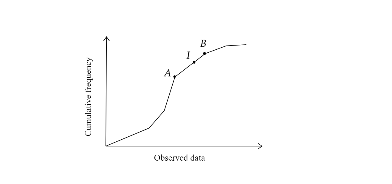
Figure 1 An ogive curve of cumulative frequency graphed against observed data.
Note that $I$ divides $\overline{AB}$ in the ratio $(R-R_i):(R_f-R)$ . Hence, the coordinates of $I$ are
\[\begin{align*}
I(x,y) &= \left(\frac{nx_1+mx_2}{m+n}, \frac{ny_1+my_2}{m+n}\right) \\
&= \left(\frac{(R_f-R)L+(R-R_i)(L+C)}{R_f - R_i}, \frac{(R_f-R)M+(R-R_i)(M+F)}{R_f - R_i}\right)\\
&= \left(L+\left(\frac{R-R_i}{R_f-R_i}\right)C, M+\left(\frac{R-R_i}{R_f-R_i}\right)F\right)
\end{align*}\]
The $x$-coordinate of $I$ is the percentile value:
\[\begin{align*}
P &= L+\left(\frac{R-R_i}{R_f-R_i}\right)C \\
&= L + \left(\frac{R - \frac{100M}{N}}{\frac{100}{N}F}\right)C \\ \therefore P &= \boxed{L + \frac{\frac{RN}{100} - M}{F}C} \end{align*}\]
and we are done. $\blacksquare$
Additional note: The $y$-coordinate tells us that $P$ is the $\left(\dfrac{RN}{100}\right)^{\mathrm{th}}$ observation.
One of the limitations of this formula is that it assumes uniform distribution in each class. This may be inaccurate for skewed or heavily concentrated data within classes. At extreme percentiles (near 0 or 100), this inaccuracy may be more apparent.
Nevertheless, if the class sizes for the grouped data were smaller, this inaccuracy decreases as linear interpolation becomes a better approximation of the actual distribution of the observed data.
Suppose we know the actual function of data distribution $f(x)$ (frequency vs data), then
\[\begin{align*}
\int^P_0{f(x)}\,dx &= \frac{RN}{100} \\
F(P) &= \frac{RN}{100} \\
P &= F^{-1}\left(\frac{RN}{100}\right)
\end{align*}\]
Mean (arithmetic mean)
We first obtain the midpoints of the classes $x_1, x_2, \dots , x_n$ where $x_i = (a_i+b_i)/2$ for all $i \in (\mathbb{Z}^+ \cap [1,n])$.
($a_i$ and $b_i$ are the lower boundary and the upper boundary of the $i$-th class respectively)
Then, the sample mean $\overline{x}$ can be estimated as follows:
\(\overline{x} = \dfrac{\sum f_ix_i}{\sum f_i}\)
where $f$ is the class frequency.
Note: This method of computing the sample mean may be inaccurate as it assumes uniform distribution within classes.
Mode
Theorem
The mode of grouped data can be estimated with the formula:
\[\text{Mode}= L + \frac{f_1-f_0}{2f_1-f_0-f_2}C\]
where
$L$ = lower boundary of modal class
$C$ = class size/interval
$f_0$ = frequency density of preceding class
$f_1$ = frequency density of modal class
$f_2$ = frequency density of succeeding class.
Equivalently,
\[\text{Mode}= L + \frac{d_1}{d_1+d_2}C\]
where $d_1 = f_1 - f_0$ and $d_2 = f_2 - f_1$.
Explanation
Suppose we plotted a histogram for our grouped data and we marked 4 points $A, B, C, D$ on the bar of the modal class (see Figure 2) as follows:
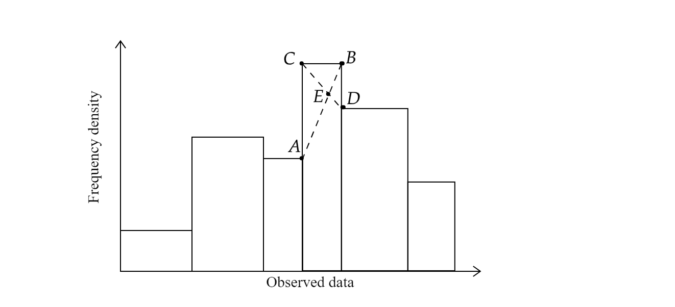
Figure 2 A histogram showing the position of five points $A,b,C,D,E$ on the bar representing the modal class.
The coordinates of the 4 points are $A(L, f_0),\,B(L+C, f_1),\, C(L, f_1),\, D(L+C, f_2)$.
Let $E$ be the point of intersection of $AB$ and $CD$. We seek to obtain the mode, which is the $x$-coordinate of $E$.
Equation of line $AB$:
\[y - f_0 = \dfrac{f_1-f_0}{C}(x-L) \dots \dots \dots (1)\]
Equation of line $CD$:
\[y - f_1 = \dfrac{f_2-f_1}{C}(x-L)\dots \dots \dots (2)\]
By solving the system of equations above, we obtain
\[\text{Mode} = \boxed{x = L + \frac{f_1-f_0}{2f_1-f_0-f_2}C}\]
and we are done. $\blacksquare$
Subsequently, we can obtain the estimated frequency density of the mode:
\[y = \frac{f_1^2-f_0f_2}{2f_1-f_0-f_2}.\]
IMPORTANT: The formulae above use $f$ to mean frequency density (NOT FREQUENCY) unless sizes of all classes are equal.
Limitations:
- Assumes uniform distribution within each class. Inaccuracies may occur if the data within classes are heavily skewed.
- Assumes symmetrical modal class.
- May not accurately represent the number of modes if there are multiple modal classes (e.g. unimodal data but multiple modal classes).